Instructor: Jimeng Sun
Introduction to Graph Analysis
In this lesson we’ll talk about graph analysis. Graph analysis, is a set of methods, that are commonly used in search engines, and social networks. And in fact, we’ll start by describing graph analysis examples, in search engine tasks. We describe some core algorithms, used likely by search engines. However, just as graph analysis can find a cluster of web pages, that are related to one another, it can also find a cluster of patients, or conditions, that are related to one another. We turn to house care applications of graph analysis, while discussing similarity graph, and spectral clustering.
Agenda
Today we’ll talk about two important graph based algorithms. First, we’ll talk about PageRank. Given a large directive graph, PageRank ranks all the node on this graph based on their importance. Second, we’ll talk about spectral clustering, which is clustering algorithm based on graph partitioning. Let’s start with PageRank.
PageRank
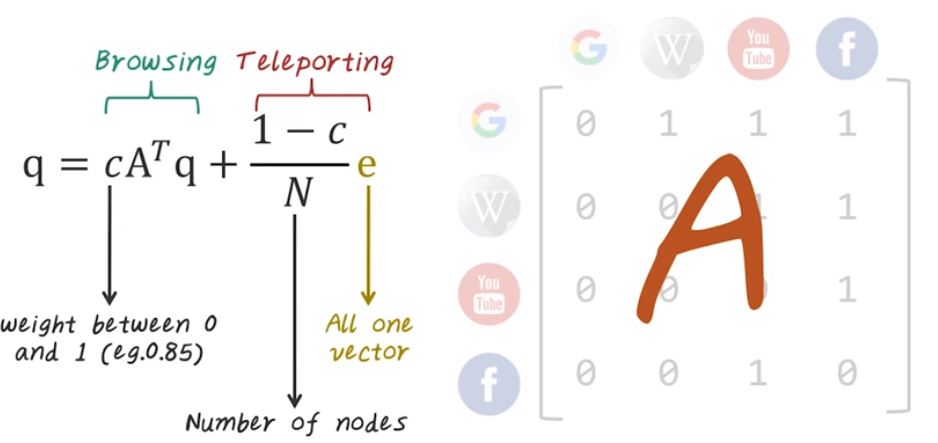
PageRank is an algorithm that was originally developed by Google’s co-founder to rank webpages. Traditional way to assess the importance of webpages is based on the content. However, content-based analysis is very susceptible to spend. And Google’s co-founders, Larry and Sergey, figured out a very smart way to rank webpages based on the link structures between the pages, instead of using the content in the page. For example, even this small directive graph, we can rank those four pages based on the link structure instead of the content inside those web pages. And the intuition behind PageRank is if more high quality page link to you, then you’re consider higher ranked. Now let’s illustrate the effect of PageRank using this example. PageRank operates on directed network, for example, given a directed graph like this, we can run PageRank algorithms to figure out what nodes are important and what nodes are not important. For example, those red nodes are considered important or higher ranked because there are many incoming edges pointing to them. And those smaller nodes are considered less important because they don’t have many node connect directly to them. And this is intuition behind PageRank algorithm. Next, let’s see how can we formulate this intuition into a mathematical algorithm. Now let’s come back to this toy example. In order to describe PageRank algorithm, we have to represent graph as a matrix. For example, this small graph will be converted to adjacency matrix to look like this. Every row represents a source and every column represents a destination. For example, for page Google, there are three outgoing links, and you can see in the adjacency matrix, we have three entries with value one. And there are two outgoing links from Wikipedia and we have two entries here corresponding to those two edges. And similarly, we can construct the rows for YouTube and Facebook that completes the adjacency matrix. And we call this matrix, A. Once we have the adjacency matrix, we can further normalize each row to make them sum to one. So every non-zero element will corresponding to a probability of jumping from the source page to the destination page. Once we have the normalized adjacency matrix A, PageRank can be described with this simple recursion. In this recursion, the q vector corresponding to all of the PageRanks, and the PageRank can be computed as the sum of these two parts, browsing and teleporting. For the browsing part, we just redistribute the old PageRank using the source destination adjacency matrix. C is the weight assigned to the browsing part, and c is a value between 0 and 1. For example, we can assign c equal to 0.85 meaning that 85% of the weight will be given to the browsing, the rest will be given to the teleporting part. The teleporting part is just randomly jump to a page. In this case, e is the all one vector and N is the number of node in the entire graph. This is mathematical definition of PageRank. Next, let’s see how we can implement this efficiently using big data systems, such as MapReduce in Hadoop.
MapReduce PageRank
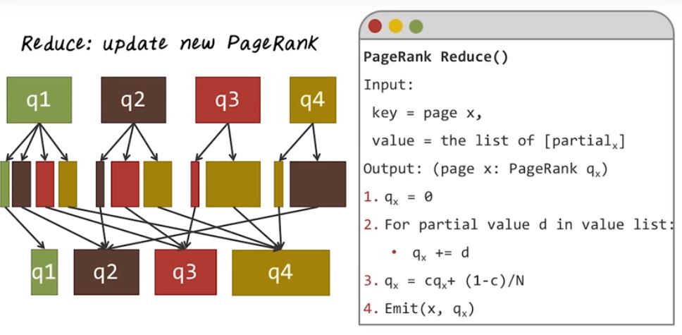
In order to implement PageRank using MapReduce, we have to partition the computation into map phase and reduce phase. So in the map phase, we’ll distribute the existing PageRank from the source to destination, following the outgoing links. Here’s a pseudocode for the map function. The input is a key value pair, where key is a webpage and the value is the current PageRank for this page qx and outgoing links y1 to ym. And output is another set of key value pairs where key is another page and value is the partial sum of the PageRank. And here’s the algorithm. We’ll first emit the page with a valid 0 to make sure all the pages are emitted. Then we follow the outgoing links. For each outgoing links we’ll emit that corresponding page, yi and distribute a portion of existing PageRank to that page. In this particular case it will be qx/m, where m is the number of outgoing links from page x. Next, let’s illustrate this map function using an example over here. In this case, we’re working with the same graph. We just reassigned the ID to each page, So, when we run the map function for each page it has its current page rank, q1, q2, q3, and q4. Now let’s look at page 1 as an example. So we know page one has three outgoing links. You can see the PageRank for q1 will be equally divided into three parts and assigned to the outgoing pages. Of course, we also emit the page itself with 0 value, and we do the same for the second page. If we look at the second page as an example, it has the two outgoing links. So we partition the existing PageRank for a second page equally and assign to those two pages. And we do the same for the third page and the fourth page. This illustrates the map phase of the algorithm for PageRank. Now let’s illustrate the reduce phase of PageRank algorithm. Here’s the pseudocode for the reduce function. The input is a key value pair and the key is a page x, and the value is a list of partial sum of the PageRank for x. The output is another key value pair, and the key is the page x and the value is the updated PageRank for x. The algorithm is quite simple, we neutralize the page rank to be 0. We sum up the partial value from the value list. That give us the PageRank from the browsing part. Next, we re-normalize this to take into account of the teleporting parts. Finally, we emit this page x and its updated PageRank, qx. So what’s happening here is the Hadoop system will perform the shuffling operation by grouping all the partial sum for each page together to get this list of partial sum of PageRanks. Then the reduce function will be applying to the list of partial sums computer updated PageRank. Now we understand the map and reduce function. To compute the final page rank we have to iteratively running this map reduce job many times in order to compute the final page rank.
Spectral Clustering
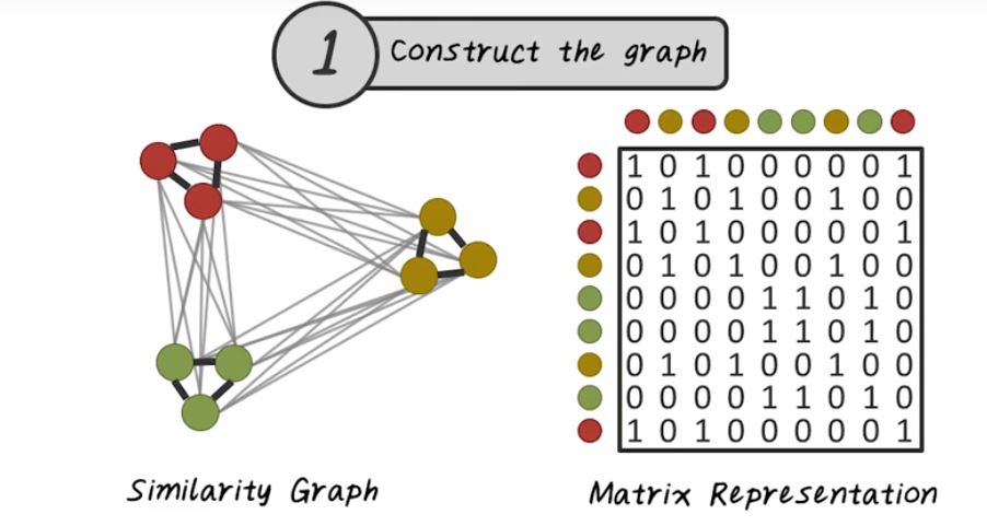
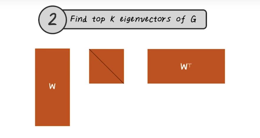
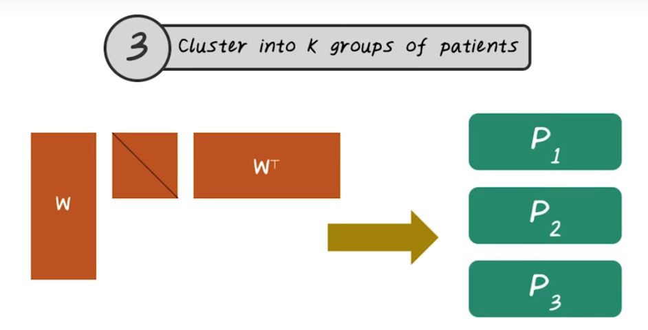
Next, let’s talk about spectral clustering. In traditional clustering algorithms, given the input data and matrix, for example this disease by patient matrix. Every row corresponding to a patient, every column corresponding to a disease. We want to learn a function, f, that partition this matrix into P1, P2, P3. Each partition corresponding to a patient cluster. In the traditional clustering setting, this function is directly applied to this matrix. While in spectral clustering this function is more involved. So next, let’s talk about how do we construct this function in the setting of spectral clustering. The first step of spectral clustering is to construct the graph. The input to the spectral clustering are patient vectors. The first step we want to connect all those patients together based on their similarity. In other words, we want to construct this similarity graph. So every node on this graph is a patient, and every edge indicates the similarity between two patients. Once we have this graph representation, we can store that efficiently using a matrix. Just like what we described in the pagerank, we can use the same adjacency matrix representation to store the similarity graph. The second step of spectral clustering is to find the top k eigen value of this graph. For example, here w represent the top k eigenvectors, and the middle matrix is the diagonal matrix with eigenvalue on the diagonal. This this third step is we want to group those patients into k groups using the eigenvectors. This is the high-level algorithm for spectral clustering. It depends on how do you implement each steps, there are many different variations of spectral clustering. Next let’s look at some of the variations.
Similarity Graph Construction
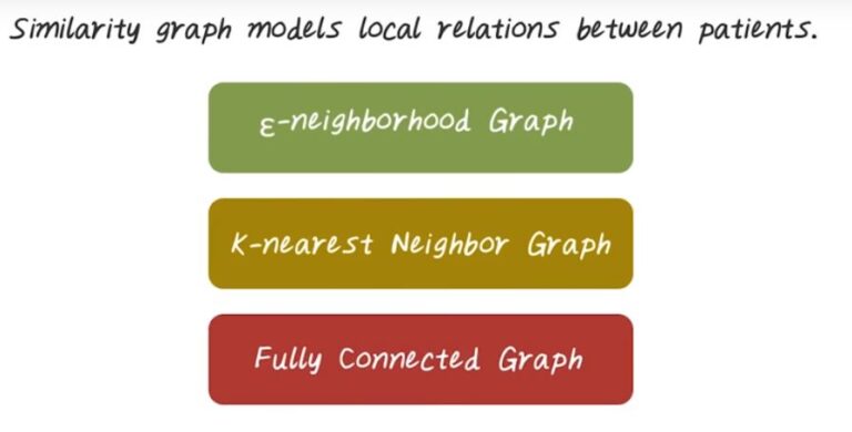
The first thing is, how do we construct the similarity graph? On high level, we want to view the similarity graph, based on the local relationship between patients. So similar patient will have a stronger relationship. There are several common ways for building such graph. We can base on epsilon neighborhood. We can use k-nearest neighbors. We can also fully connect the graph, but assign a different way to the address. Next, let’s look at them in more details.
E-Neighborhood Graph
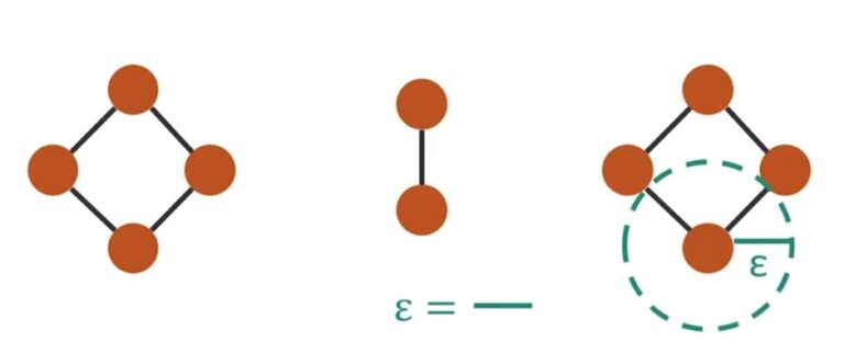
Let’s start with Epsilon Neighborhood Graph. Let’s illustrate the idea using this example. Every node here indicate a patient, and in this example we have ten patients. For Epsilon Neighborhood Graph, what we are going to do here is, we’ll connect patients if they are within epsilon distance to each other. For example, this two patients are within epsilon distance, so an edge formed between them. But the distance between these two patients is greater than epsilon, so there’s no edge between them. In this case, the epsilon is indicated by this length.
K-Nearest Neighbor Graph
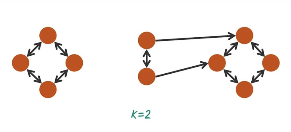
Another way to compute similarity graph is based on K-nearest Neighbor Search. For example we have this 10 patient over here. We want to perform K-nearest neighbor search from each patient and the resulting graph is this directed graph indicate the two nearest neighbor from each node. For example the two nearest neighbor of this patient are this one and this one. So one benefit of this k-nearest neighbor graph is the graph can be very sparse when the k is small, and there is several different variation of such graph. For example, we can have the edge to be binary, just zero and one, or we can actually assign different ways based on the distance between those two neighbors.
Fully Connected Graph
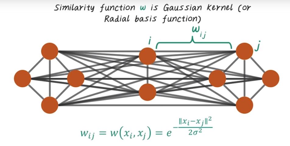
Another way to construct the similarity graph is to just use the fully connected graph, but parameterize the edges differently, based on similarity. For example, for this ten patients, we can connect everybody to everybody, have this fully connected graph. Then the edge wave will be determined by this Gaussian kernel or this Radial based function. For example the edge wave, Wij between those two patients, can be computed using this formula, which indicate the Gaussian kernel.
Spectral Clustering Algorithm
So far, we explained the high level ideas of spectral clusterings. Depending on how you implement each steps, there are many different variations. If you want to learn more about different variation of spectral clusterings, please refer to this tutorial, and to learn about all those different variations. For example, we can have this very simple unnormalized spectral clusterings, just involve building the graph compute eigenvectors, then perform k-mean clusters on those eigenvectors. This is probably the simplest spectral clustering algorithms out there. Then there are different enhancement on the original algorithms, by normalizing the graph differently. For example this normalized spectral clusterings published in 2000 and another different normalized spectral clusterings published in 2002. Spectral clustering perform really well in practice even when the data are high dimensional or noisy. In fact, there are very good theoretical foundation behind spectral clustering. If you are interested in learning more, you can refer to this paper. In that paper, they actually illustrate theoretically why spectral clustering works. Intuitively speaking, if the data are not really clusterable in the original space. By performing the spectral clustering, you can transform the original data into the space where the clusters are well defined. So for example here, the color indicate different clusters, in the original space, it’s very difficult to carve out these three clusters. But when you perform spectral clustering, in the eigenspace you can find all those three clusters are well separated.